Generative Adversarial Networks

Note: Still updating..

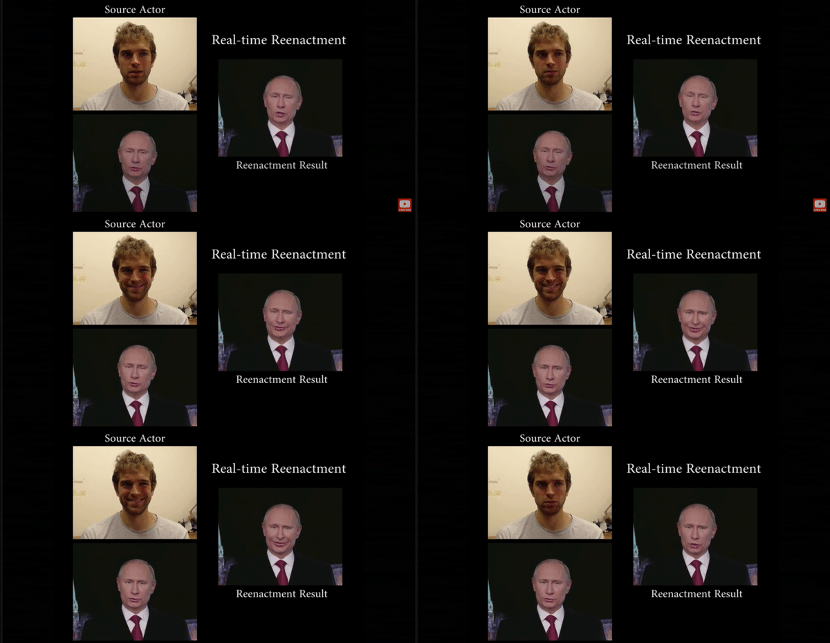
GAN is about generating data from scratch, like an artist. The modern GAN usage would involve generating data, like composing a symphony, or drawing a landscape. Thousands of GAN research papers were published in recent years, with broad areas ranging from game development, medical imaging, text-to-image translation, etc.

Some Preliminaries

• Probabilistic Generative Models
  • e.g. MLE estimation for continuous input features
• Probabilistic Discriminative Models
  • e.g. multiclass logistic regression
• Neural Network Basics
  • Multilayer Perceptrons
  • Backpropagation

How Do the Adversarial Nets work?

The GAN provides a framework for estimating generative models through an adversarial process. In this framework we train the following two models simultaneously:

• \(G\) - Generative model that captures the data distribution.
• \(D\) - Discriminative model that estimates the probability that a sample is from the training data, rather than \(G\).

To learn \(G\)’s generated distrbution \(p_g\) from data input \(\mathbf{x}\), we define a prior on the input noise variables \(p_{\mathbf{z}}(\mathbf{z})\), then we use a differentiable function \(G\) to map \(\mathbf{z}\) to the data space as \(G(\mathbf{z};\theta_g)\).

• Here \(G\) is being represented by a multilayer perceptron with parameters \(\theta_g\).

Additionally, we define another multilayer perceptron \(D(\mathbf{x};\theta_d)\) that outputs a scalar.

• Here \(D(\mathbf{x})\) represents the probability that \(\mathbf{x}\) coming from the data, rather than the generated \(p_g\).

Finally, our goal is to train \(D\) to maximize the probability of assigning the correct label to both samples from \(G\) and training examples. Therefore, we will train \(G\) to minimize \(\log(1-D(G(\mathbf{z})))\). This yields a two-player minimax game with value function \(V(G,D)\):

Note that in the function space of arbitrary \(G\) and \(D\), there exists a unique solution, in which \(G\) recovers the training data distribution, and \(D\) will be constantly \(1/2\).

If \(G\) and \(D\) are defined as multilayer perceptrons, we then are able to train the system using backpropagation.

A Pedagogical Explanation

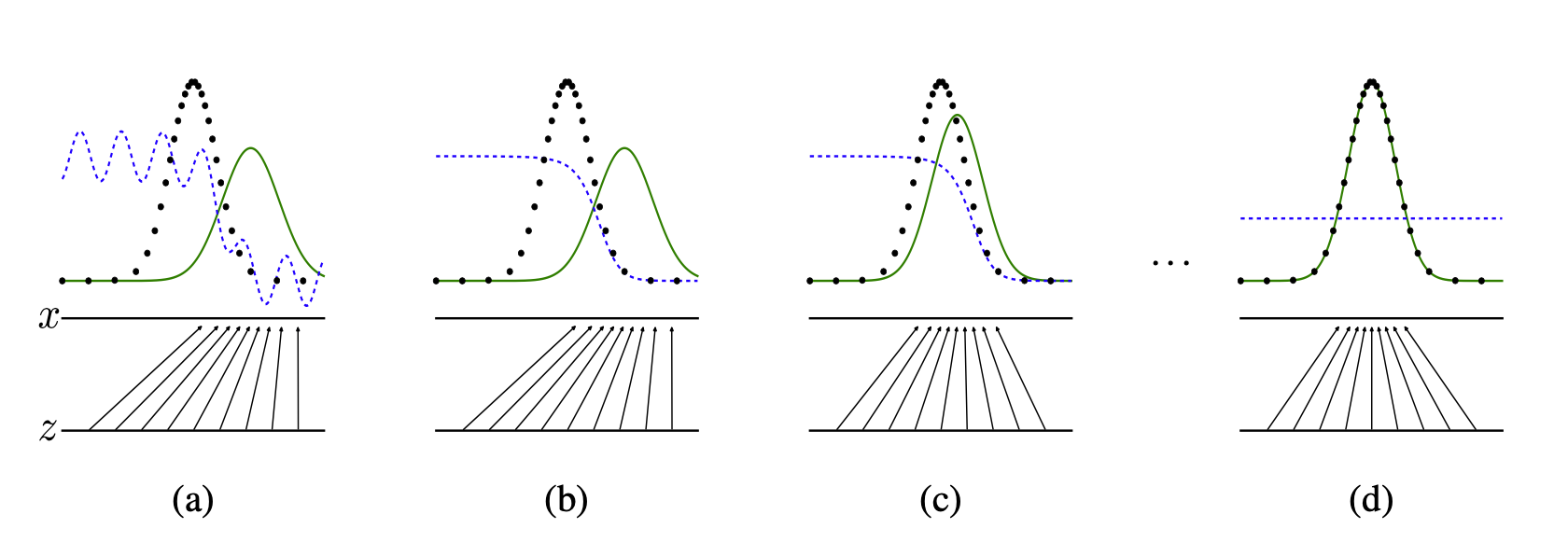
This figure illustrate generative adverserial nets trained by simultaneously updating the discriminative distribution (\(D\), blue, dashed line), so that it discriminates between samples from the data generating distribution \(p_{\mathbf{x}}\) (black, dotted line) from the generative distribution \(p_g(G)\) (green, solid line).

• The lower horizontal line is the domain from which \(\mathbf{z}\) is sampled (uniformly, in this case);
• The upper horizontal line is part of the domain of \(\mathbf{x}\);
• The upward arrows show how the mapping \(\mathbf{x}=G(\mathbf{z})\) imposes the non-uniform distribution \(p_g\) on transformed samples.
• \(G\) contracts in regions of high density, and expands in regions of low density of \(p_g\).

a) Consider an adversarial pair near convergence: \(p_g\) is similar to \(p_{\text{data}}\), and \(D\) is a partially accurate classifier.

b) In the inner loop of the algorithm, \(D\) is trained to discriminate samples from the data. It converges to

c) After an update to \(G\), the gradient of \(D\) has guided \(G(\mathbf{z})\) to flow to regions that are more likely to be classified as data.

d) After a few steps of training, if \(G\) and \(D\) have enough capacity, they will reach a point where both cannot improve, since \(p_g=p_{\text{data}}\).

Note that At this stage, the discriminator is unable to differentiate between the two distributions, i.e. \(D(\mathbf{x})=1/2\).

An Analogy…

To view this in a analogous way, try to think in the following way:

• Consider the generative model \(G\) as a group of counterfeiters trying to produce fake paintings without being detected.

• Consider the discriminative model \(D\) as a group of police trying to detect the fake paintings.

Then the competition will drive both groups to improve their methods until the counterfeits draw paintings that are not disguinshable from the actual paintings anymore.

Example Showcase

Related work

• Check out Ian Goodfellow’s tutorial workshop.

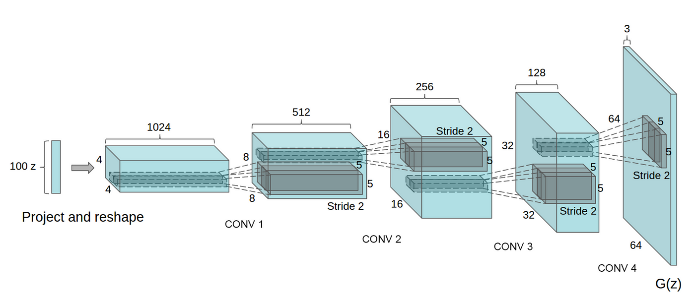
• The following image illustrates the DCGAN (Radford et al.), one of the most popular generator network design, which performes multiple transposed convolutions to upsample \(\mathbf{z}\) to generate the data \(\mathbf{x}\) (here, an image).

References

[1] Goodfellow, I. J., Pouget-Abadie, J., Mirza, M., Xu, B., Warde-Farley, D., Ozair, S., Courville, A., & Bengio, Y. (2014). Generative Adversarial Networks. ArXiv:1406.2661 [Cs, Stat]. http://arxiv.org/abs/1406.2661

[2] Radford, A., Metz, L., & Chintala, S. (2015). Unsupervised representation learning with deep convolutional generative adversarial networks. arXiv preprint arXiv:1511.06434.